Visualizing U.S. census data with custom variables is quite difficult. Google Maps is a great visualization tool. If we could overlay data on the map, it would be delicious. We can! Google Fusion Tables allows you to upload custom data to display on the map. The hard part is getting the coordinate points that form a polygon for every county in the U.S. (and knowing what counties are in each state)
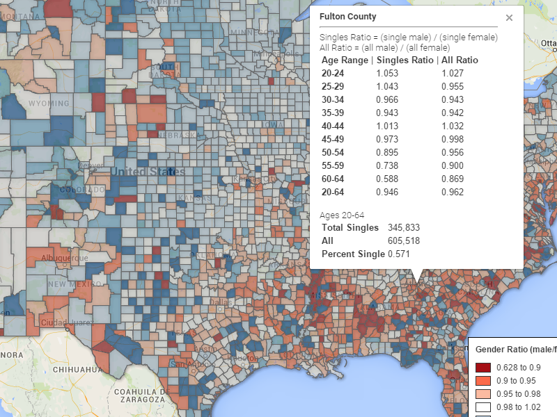
The following map is the end result of this tutorial. It’s a map of gender ratios in every county. The colors are based on the gender ratio of all people ages 20-64. The info-window (click a county) shows a detailed breakdown by age of the gender ratio of all people and single people. I chose these variables because I already used them in my Best Places to Find a Date report.
Map of Gender Ratios VIEW FULL SCREEN (click a county for more info)
HISTOGRAMS
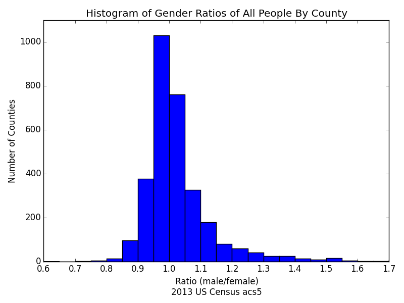
The following is a histogram of gender ratios for all people in the 20-64 age range for all counties. Carefully note that it is by county meaning that a county with millions and a county with just hundreds of people get just one vote. It is narrowly centered at a 1:1 ratio (1 male per female.)
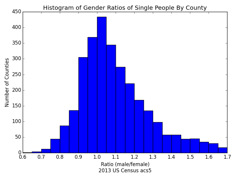
The following is a histogram of gender ratios of SINGLE people by county. There is a palpable difference from the first histogram considering the data is from the same source. What’s going on here? It’s a beautiful illustration of age disparity in relationships (assumes relationships are heterosexual.) There is allot of demand for young women from young & older men. As a result, older single women are rather lonely (see graph below.)
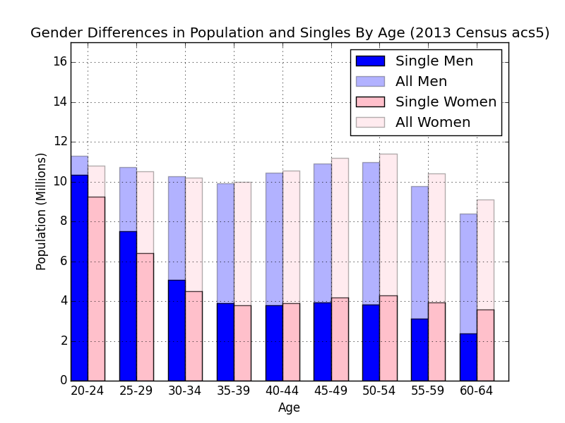
The following chart is packed with information. The absolute gender ratio by age, the gender ratio of single people by age, and the ratio of married people by age. The ratio for singles in the 20-24 age range is 1.12 (male/female) and in the 60-64 age range it’s 0.67. If you would like to reproduce this chart (not in the tutorial), here is a link to the text of the Python script I wrote to create it.
TUTORIAL
Here is the GitHub Source Code (you will need the KML JSON file ~22MB)
__author__ = 'Thomaz L Santana'
# Tutorial for Python 3
import matplotlib.pyplot as plt
import urllib.request
import functools
import ast
import json
import us
import humanize


# Now load the kml data needed to make this work...
# Or if you would like to create your own https://www.census.gov/geo/maps-data/data/cbf/cbf_counties.html
file = open('state-county-fips-kml-json.txt', 'r')
gz = json.loads(file.read())

# state FIPS (federal information processing standard)
state_fips = us.states.mapping('fips', 'name')
# remove American territories so that we only have states
for item in [None, '72', '66', '69', '60', '78']:
    del state_fips[item]


# Here is the documentation, datasets available, variables, and more... http://api.census.gov/data.html
class Census:
    def __init__(self, key):
        self.key = key

    def get(self, fields, geo, year=2013, dataset='acs5'):
        fields = [','.join(fields)]
        base_url = 'http://api.census.gov/data/%s/%s?key=%s&get=' % (str(year), dataset, self.key)
        query = fields
        for item in geo:
            query.append(item)
        add_url = '&'.join(query)
        url = base_url + add_url
        req = urllib.request.Request(url)
        response = urllib.request.urlopen(req)
        return ast.literal_eval(response.read().decode('utf8'))


# Get a Census API Key http://api.census.gov/data/key_signup.html
# enter your name or NA for 'Organization Name'
c = Census('YOUR-KEY-HERE')
Here is the main documentation for the census API. The Census class is rather simple so that anyone can look at example census api queries and figure out how to ask for what they want. The list of variables for the 2013 acs5 dataset is very, very long and takes minutes to load. You will need a Census API Key (get key.) You can just enter your name or whatever for Organization Name.
# Now have a look at the variables available for the 2013 acs5 dataset
# http://api.census.gov/data/2013/acs5/variables.html
# Wow that took long to load...

# Let's create a map to visualize the gender ratio of single people in the US
# Hum... I'm not sure if married people who say they are separated count as single people but lets include them

# Male never married: 20-24, 25-29, 30-34, 35-39, 40-44, 45-49, 50-54, 55-59, 60-64
# Male widowed: 20-24, 25-29, 30-34, 35-39, 40-44, 45-49, 50-54, 55-59, 60-64
# Male divorced: 20-24, 25-29, 30-34, 35-39, 40-44, 45-49, 50-54, 55-59, 60-64
# Male married but separated: 20-24, 25-29, 30-34, 35-39, 40-44, 45-49, 50-54, 55-59, 60-64
single_data_m = ['B12002_006E', 'B12002_007E', 'B12002_008E', 'B12002_009E', 'B12002_010E', 'B12002_011E', 'B12002_012E', 'B12002_013E', 'B12002_014E',
                 'B12002_068E', 'B12002_069E', 'B12002_070E', 'B12002_071E', 'B12002_072E', 'B12002_073E', 'B12002_074E', 'B12002_075E', 'B12002_076E',
                 'B12002_083E', 'B12002_084E', 'B12002_085E', 'B12002_086E', 'B12002_087E', 'B12002_088E', 'B12002_089E', 'B12002_090E', 'B12002_091E',
                 'B12002_038E', 'B12002_039E', 'B12002_040E', 'B12002_041E', 'B12002_042E', 'B12002_043E', 'B12002_044E', 'B12002_045E', 'B12002_046E']

# Female never married: 20-24, 25-29, 30-34, 35-39, 40-44, 45-49, 50-54, 55-59, 60-64
# Female widowed: 20-24, 25-29, 30-34, 35-39, 40-44, 45-49, 50-54, 55-59, 60-64
# Female divorced: 20-24, 25-29, 30-34, 35-39, 40-44, 45-49, 50-54, 55-59, 60-64
# Female married but separated: 20-24, 25-29, 30-34, 35-39, 40-44, 45-49, 50-54, 55-59, 60-64
single_data_f = ['B12002_099E', 'B12002_100E', 'B12002_101E', 'B12002_102E', 'B12002_103E', 'B12002_104E', 'B12002_105E', 'B12002_106E', 'B12002_107E',
                 'B12002_161E', 'B12002_162E', 'B12002_163E', 'B12002_164E', 'B12002_165E', 'B12002_166E', 'B12002_167E', 'B12002_168E', 'B12002_169E',
                 'B12002_176E', 'B12002_177E', 'B12002_178E', 'B12002_179E', 'B12002_180E', 'B12002_181E', 'B12002_182E', 'B12002_183E', 'B12002_184E',
                 'B12002_131E', 'B12002_132E', 'B12002_133E', 'B12002_134E', 'B12002_135E', 'B12002_136E', 'B12002_137E', 'B12002_138E', 'B12002_139E']

# Now let's get the absolute gender so no one goes crazy thinking the US is overflowing with men
# Male 20, 21, 22-24, 25-29, 30-34, 35-39, 40-44, 45-49, 50-54, 55-59, 60-61, 62-64
# Female 20, 21, 22-24, 25-29, 30-34, 35-39, 40-44, 45-49, 50-54, 55-59, 60-61, 62-64
gender_data = ['B01001_008E', 'B01001_009E', 'B01001_010E', 'B01001_011E', 'B01001_012E', 'B01001_013E', 'B01001_014E', 'B01001_015E', 'B01001_016E', 'B01001_017E', 'B01001_018E', 'B01001_019E',
               'B01001_032E', 'B01001_033E', 'B01001_034E', 'B01001_035E', 'B01001_036E', 'B01001_037E', 'B01001_038E', 'B01001_039E', 'B01001_040E', 'B01001_041E', 'B01001_042E', 'B01001_043E']
This may be the most tedious part – gathering all the census variables you want to use.
# Now the onerous task of compiling these data
def compile_county(single_m, single_f, all_mf):
    dic = {}
    # All male by age
    dic['m20'] = int(all_mf[0]) + int(all_mf[1]) + int(all_mf[2])
    dic['m25'] = int(all_mf[3])
    dic['m30'] = int(all_mf[4])
    dic['m35'] = int(all_mf[5])
    dic['m40'] = int(all_mf[6])
    dic['m45'] = int(all_mf[7])
    dic['m50'] = int(all_mf[8])
    dic['m55'] = int(all_mf[9])
    dic['m60'] = int(all_mf[10]) + int(all_mf[11])
    dic['m'] = dic['m20'] + dic['m25'] + dic['m30'] + dic['m35'] + dic['m40'] + dic['m45'] + dic['m50'] + dic['m55'] + dic['m60']
    # All female by age
    dic['f20'] = int(all_mf[12]) + int(all_mf[13]) + int(all_mf[14])
    dic['f25'] = int(all_mf[15])
    dic['f30'] = int(all_mf[16])
    dic['f35'] = int(all_mf[17])
    dic['f40'] = int(all_mf[18])
    dic['f45'] = int(all_mf[19])
    dic['f50'] = int(all_mf[20])
    dic['f55'] = int(all_mf[21])
    dic['f60'] = int(all_mf[22]) + int(all_mf[23])
    dic['f'] = dic['f20'] + dic['f25'] + dic['f30'] + dic['f35'] + dic['f40'] + dic['f45'] + dic['f50'] + dic['f55'] + dic['f60']
    # Male never married, widowed, divorced, married but separated - sum by age
    data = [single_m[x] for x in range(0, 28, 9)]
    dic['m_single20'] = functools.reduce(lambda x, y: int(x)+int(y), data)
    data = [single_m[x] for x in range(1, 29, 9)]
    dic['m_single25'] = functools.reduce(lambda x, y: int(x)+int(y), data)
    data = [single_m[x] for x in range(2, 30, 9)]
    dic['m_single30'] = functools.reduce(lambda x, y: int(x)+int(y), data)
    data = [single_m[x] for x in range(3, 31, 9)]
    dic['m_single35'] = functools.reduce(lambda x, y: int(x)+int(y), data)
    data = [single_m[x] for x in range(4, 32, 9)]
    dic['m_single40'] = functools.reduce(lambda x, y: int(x)+int(y), data)
    data = [single_m[x] for x in range(5, 33, 9)]
    dic['m_single45'] = functools.reduce(lambda x, y: int(x)+int(y), data)
    data = [single_m[x] for x in range(6, 34, 9)]
    dic['m_single50'] = functools.reduce(lambda x, y: int(x)+int(y), data)
    data = [single_m[x] for x in range(7, 35, 9)]
    dic['m_single55'] = functools.reduce(lambda x, y: int(x)+int(y), data)
    data = [single_m[x] for x in range(8, 36, 9)]
    dic['m_single60'] = functools.reduce(lambda x, y: int(x)+int(y), data)
    dic['m_single'] = dic['m_single20'] + dic['m_single25'] + dic['m_single30'] + dic['m_single35'] + \
                      dic['m_single40'] + dic['m_single45'] + dic['m_single50'] + dic['m_single55'] + dic['m_single60']
    # Female never married, widowed, divorced, married but separated - sum by age
    data = [single_f[x] for x in range(0, 28, 9)]
    dic['f_single20'] = functools.reduce(lambda x, y: int(x)+int(y), data)
    data = [single_f[x] for x in range(1, 29, 9)]
    dic['f_single25'] = functools.reduce(lambda x, y: int(x)+int(y), data)
    data = [single_f[x] for x in range(2, 30, 9)]
    dic['f_single30'] = functools.reduce(lambda x, y: int(x)+int(y), data)
    data = [single_f[x] for x in range(3, 31, 9)]
    dic['f_single35'] = functools.reduce(lambda x, y: int(x)+int(y), data)
    data = [single_f[x] for x in range(4, 32, 9)]
    dic['f_single40'] = functools.reduce(lambda x, y: int(x)+int(y), data)
    data = [single_f[x] for x in range(5, 33, 9)]
    dic['f_single45'] = functools.reduce(lambda x, y: int(x)+int(y), data)
    data = [single_f[x] for x in range(6, 34, 9)]
    dic['f_single50'] = functools.reduce(lambda x, y: int(x)+int(y), data)
    data = [single_f[x] for x in range(7, 35, 9)]
    dic['f_single55'] = functools.reduce(lambda x, y: int(x)+int(y), data)
    data = [single_f[x] for x in range(8, 36, 9)]
    dic['f_single60'] = functools.reduce(lambda x, y: int(x)+int(y), data)
    dic['f_single'] = dic['f_single20'] + dic['f_single25'] + dic['f_single30'] + dic['f_single35'] + \
                      dic['f_single40'] + dic['f_single45'] + dic['f_single50'] + dic['f_single55'] + dic['f_single60']
    return dic
In Python 2.x the ‘reduce’ function is just there but in Python 3.x you have to import functools… what a shame, it’s so useful.
census_dic = {}
for state in state_fips.keys():
    # Get data for all counties '*' in state
    single_m_result = c.get(single_data_m, ['in=state:%s' % state, 'for=county:%s' % '*'])
    single_f_result = c.get(single_data_f, ['in=state:%s' % state, 'for=county:%s' % '*'])
    all_result = c.get(gender_data, ['in=state:%s' % state, 'for=county:%s' % '*'])

    census_dic[state] = {}
    num_counties_in_state = len(all_result)
    # compile county data by age
    for i in range(1, num_counties_in_state):
        # county fips any [-1] from the results will do
        county_fips = all_result[i][-1]
        compiled_data = compile_county(single_m_result[i], single_f_result[i], all_result[i])
        census_dic[state][county_fips] = compiled_data
        # Now add the gazetteer kml shapefile and county name
        try:
            census_dic[state][county_fips]['kml'] = gz[state][county_fips]['kml']
            census_dic[state][county_fips]['name'] = gz[state][county_fips]['name']
        except KeyError:
            # Virginia is a complicated place... no shapefile for county fips 515 yet census data for it, wth
            # Also no record of county 515 http://en.wikipedia.org/wiki/List_of_counties_in_Virginia wth**2
            # lets delete it
            del census_dic[state][county_fips]
The code above makes requests to the census api for the variable we (I) want for each state. The census (and the kml json in source code) uses FIPS codes. For example ‘41051’ where the first two characters represent the state ’41’ is Oregon and the last three represent the county ‘051’ is Multnomah County (the county of Portland.) To go in a bit deeper ‘59000’ is the fips of the city of Portland but it gets complicated because the boundary of some cities overlap with more than one county e.g. New York City stuff like this makes GIS analyses difficult.
# Some more data compilation
singles_ratios_plot = []
all_ratios_plot = []
# iterate through states
for k, v in census_dic.items():
    # iterate through counties in state
    for k2, v2 in v.items():
        singles_ratios_plot.append(v2['m_single'] / v2['f_single'])
        # all_ratios_plot.append(v2['m'] / v2['f'])
        m = v2['m20'] + v2['m25'] + v2['m30'] + v2['m35'] + v2['m40'] + v2['m45'] + v2['m50'] + v2['m55'] + v2['m60']
        f = v2['f20'] + v2['f25'] + v2['f30'] + v2['f35'] + v2['f40'] + v2['f45'] + v2['f50'] + v2['f55'] + v2['f60']
        all_ratios_plot.append(m / f)


# While we're at it let's make some histograms...
bins = [x*0.05 for x in range(12, 36)]
xticks = [bins[x] for x in range(0, len(bins), 2)]

# Single Plot
plt.hist(singles_ratios_plot, bins=bins, facecolor='blue')
plt.xticks(xticks)
plt.xlim([0.6, 1.7])
plt.xlabel('Ratio (male/female)\n2013 US Census acs5')
plt.ylabel('Number of Counties')
plt.title('Histogram of Gender Ratios of Single People By County')
plt.tight_layout()
# plt.show()
plt.savefig('Histogram_of_Gender_Ratios_of_Single_People.png')

# All plot
plt.hist(all_ratios_plot, bins=bins, facecolor='blue')
plt.xticks(xticks)
plt.xlim([0.6, 1.7])
plt.ylim([0, 1100])
plt.xlabel('Ratio (male/female)\n2013 US Census acs5')
plt.ylabel('Number of Counties')
plt.title('Histogram of Gender Ratios of All People By County')
plt.tight_layout()
# plt.show()
plt.savefig('Histogram_of_Gender_Ratios_of_All_People.png')
I went on a tangent here but I thought it was a great way to visualize the age disparity in relationships.
# Create the tedious CSV to upload... gotta be fastidious
sList = ['"countyName","s20","s25","s30","s35","s40","s45","s50","s55","s60","a20","a25","a30","a35","a40","a45","a50","a55","a60","singleR","allR","singles_count","all_count","singles_ratio","kml"']
# iterate through states
for k, v in census_dic.items():
    # iterate through counties in state
    for k2, v2 in v.items():
        # Singles ratios
        try:
            s20 = '%.3f' % (census_dic[k][k2]['m_single20'] / census_dic[k][k2]['f_single20'])
        except ZeroDivisionError:
            s20 = 'NA'
        try:
            s25 = '%.3f' % (census_dic[k][k2]['m_single25'] / census_dic[k][k2]['f_single25'])
        except ZeroDivisionError:
            s25 = 'NA'
        try:
            s30 = '%.3f' % (census_dic[k][k2]['m_single30'] / census_dic[k][k2]['f_single30'])
        except ZeroDivisionError:
            s30 = 'NA'
        try:
            s35 = '%.3f' % (census_dic[k][k2]['m_single35'] / census_dic[k][k2]['f_single35'])
        except ZeroDivisionError:
            s35 = 'NA'
        try:
            s40 = '%.3f' % (census_dic[k][k2]['m_single40'] / census_dic[k][k2]['f_single40'])
        except ZeroDivisionError:
            s40 = 'NA'
        try:
            s45 = '%.3f' % (census_dic[k][k2]['m_single45'] / census_dic[k][k2]['f_single45'])
        except ZeroDivisionError:
            s45 = 'NA'
        try:
            s50 = '%.3f' % (census_dic[k][k2]['m_single50'] / census_dic[k][k2]['f_single50'])
        except ZeroDivisionError:
            s50 = 'NA'
        try:
            s55 = '%.3f' % (census_dic[k][k2]['m_single55'] / census_dic[k][k2]['f_single55'])
        except ZeroDivisionError:
            s55 = 'NA'
        try:
            s60 = '%.3f' % (census_dic[k][k2]['m_single60'] / census_dic[k][k2]['f_single60'])
        except ZeroDivisionError:
            s60 = 'NA'
        # all ratios
        try:
            a20 = '%.3f' % (census_dic[k][k2]['m20'] / census_dic[k][k2]['f20'])
        except ZeroDivisionError:
            a20 = 'NA'
        try:
            a25 = '%.3f' % (census_dic[k][k2]['m25'] / census_dic[k][k2]['f25'])
        except ZeroDivisionError:
            a25 = 'NA'
        try:
            a30 = '%.3f' % (census_dic[k][k2]['m30'] / census_dic[k][k2]['f30'])
        except ZeroDivisionError:
            a30 = 'NA'
        try:
            a35 = '%.3f' % (census_dic[k][k2]['m35'] / census_dic[k][k2]['f35'])
        except ZeroDivisionError:
            a35 = 'NA'
        try:
            a40 = '%.3f' % (census_dic[k][k2]['m40'] / census_dic[k][k2]['f40'])
        except ZeroDivisionError:
            a40 = 'NA'
        try:
            a45 = '%.3f' % (census_dic[k][k2]['m45'] / census_dic[k][k2]['f45'])
        except ZeroDivisionError:
            a45 = 'NA'
        try:
            a50 = '%.3f' % (census_dic[k][k2]['m50'] / census_dic[k][k2]['f50'])
        except ZeroDivisionError:
            a50 = 'NA'
        try:
            a55 = '%.3f' % (census_dic[k][k2]['m55'] / census_dic[k][k2]['f55'])
        except ZeroDivisionError:
            a55 = 'NA'
        try:
            a60 = '%.3f' % (census_dic[k][k2]['m60'] / census_dic[k][k2]['f60'])
        except ZeroDivisionError:
            a60 = 'NA'
        # singles ratio
        singleR = '%.3f' % (census_dic[k][k2]['m_single'] / census_dic[k][k2]['f_single'])
        # all ratio
        allR = '%.3f' % (census_dic[k][k2]['m'] / census_dic[k][k2]['f'])
        # gazetteer info
        kml = census_dic[k][k2]['kml']
        name = census_dic[k][k2]['name']
        # extra info
        singles_count = humanize.intcomma(census_dic[k][k2]['m_single'] + census_dic[k][k2]['f_single'])
        all_count = humanize.intcomma(census_dic[k][k2]['m'] + census_dic[k][k2]['f'])
        singles_ratio = '%.3f' % ((census_dic[k][k2]['m_single'] + census_dic[k][k2]['f_single']) / (census_dic[k][k2]['m'] + census_dic[k][k2]['f']))
        # create a CSV row
        variables = [name, s20, s25, s30, s35, s40, s45, s50, s55, s60, a20, a25, a30, a35, a40, a45, a50, a55, a60,
                     singleR, allR, singles_count, all_count, singles_ratio, kml]
        s = ''.join(['"%s",' % x for x in variables])
        sList.append(s)

# make the CSV to upload to Google Fusion Tables
fusionTableCSV = '\n'.join(sList)
file = open('census_ratios_fusion_table.csv', 'w')
file.write(fusionTableCSV)
Finally done with the coding. There are ‘try’ and ‘except’ everywhere because we have no guarantee that there is anyone for the selected variable in a county.
Now that we have the CSV file (~23MB) full of juicy-delicious data and KML shapefiles we turn to Google Fusion Tables. You need an account on Google.
Go to your Google Drive, click new then ‘more’ and there is no Fusion Tables if you have never done this before.

Click ‘Connect more apps’ and search ‘fusion tables’ (image below)

Click ‘Connect’ to add the app to your Google Drive. Now that you have the Google Fusion Tables app click ‘NEW’ again and go to ‘more’ to see Fusion Tables.

Click NEW Google Fusion Tables to add the CSV you just created.
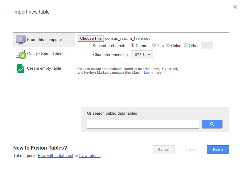
The file is a CSV so leave the separator character as comma and click next. Note it’s a ~23MB file so it will take a bit to load.
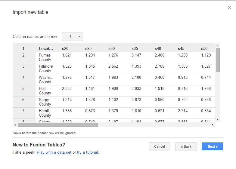
So far so good… click next.
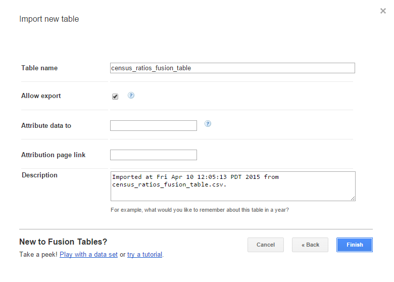
Now enter the name of the table and a description and finish.
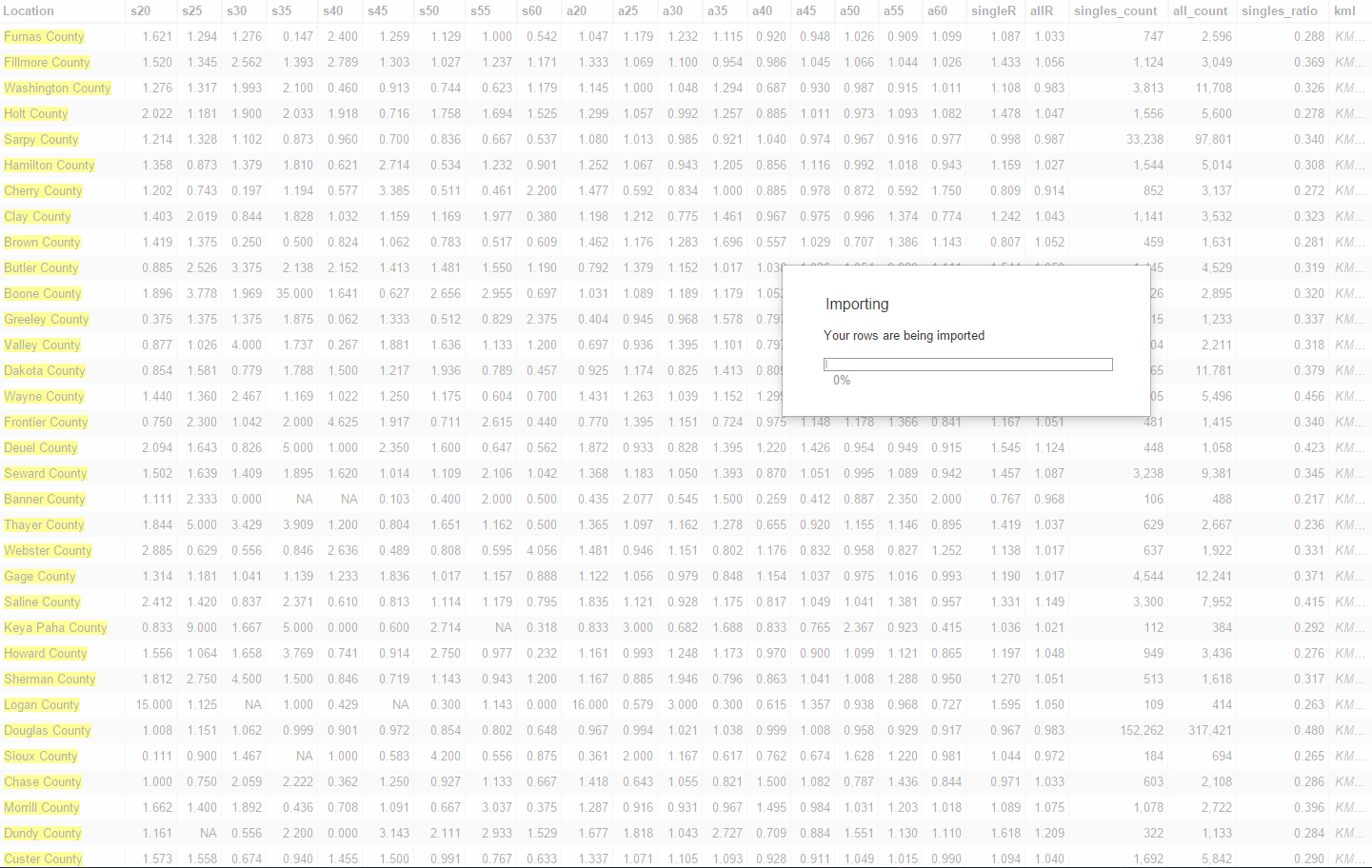
Wait a bit for Google to work some magic. Then switch from the ‘Rows’ tab to the ‘Map’ tab.
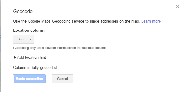
Then click ‘Pause geocoding’ and switch the ‘Location column’ to the ‘kml’ column in the CSV we uploaded. After switching to kml column and geocoding I think you just click cancel to exit that screen.
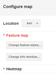
Then on the left make sure you have ‘Location’ set as kml column.
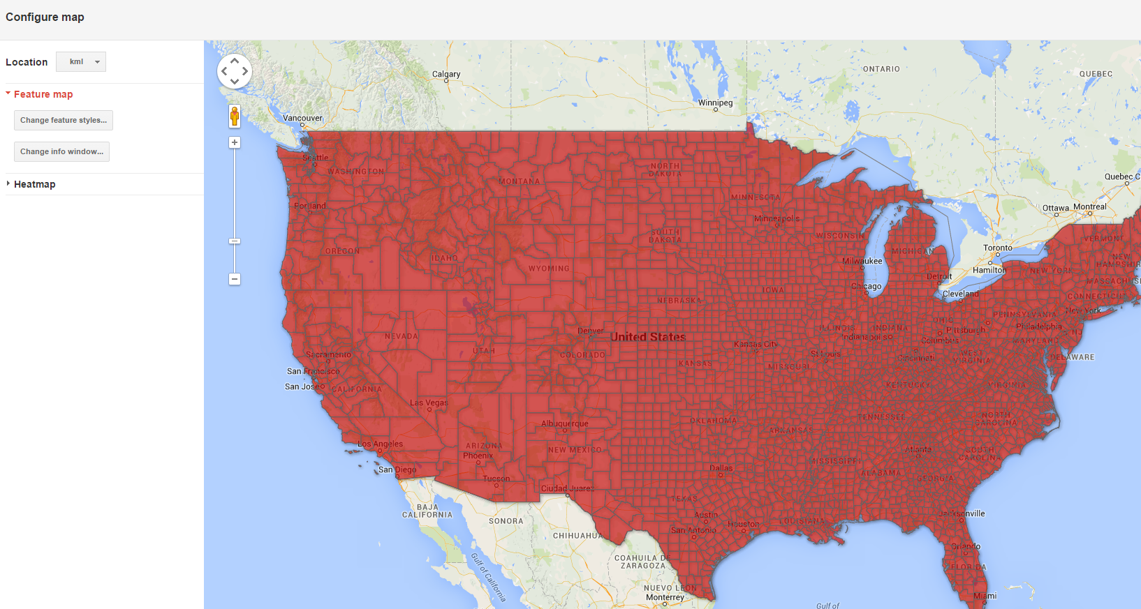
This is what you should see now… an innocuous map conveying no information.
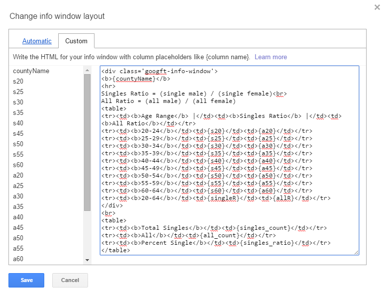
On the left click ‘Change info window’ and edit what you want to display when you click a county.
Here is what I have:
<div class='googft-info-window'>
<b>{countyName}</b>
<hr>
Singles Ratio = (single male) / (single female)<br>
All Ratio = (all male) / (all female)
<table>
<tr><td><b>Age Range</b> |</td><td><b>Singles Ratio</b> |</td><td><b>All Ratio</b></td></tr>
<tr><td><b>20-24</b></td><td>{s20}</td><td>{a20}</td></tr>
<tr><td><b>25-29</b></td><td>{s25}</td><td>{a25}</td></tr>
<tr><td><b>30-34</b></td><td>{s30}</td><td>{a30}</td></tr>
<tr><td><b>35-39</b></td><td>{s35}</td><td>{a35}</td></tr>
<tr><td><b>40-44</b></td><td>{s40}</td><td>{a40}</td></tr>
<tr><td><b>45-49</b></td><td>{s45}</td><td>{a45}</td></tr>
<tr><td><b>50-54</b></td><td>{s50}</td><td>{a50}</td></tr>
<tr><td><b>55-59</b></td><td>{s55}</td><td>{a55}</td></tr>
<tr><td><b>60-64</b></td><td>{s60}</td><td>{a60}</td></tr>
<tr><td><b>20-64</b></td><td>{singleR}</td><td>{allR}</td></tr>
</div>
<br>
Ages 20-64
<table>
<tr><td><b>Total Singles</b></td><td>{singles_count}</td></tr>
<tr><td><b>All</b></td><td>{all_count}</td></tr>
<tr><td><b>Percent Single</b></td><td>{singles_ratio}</td></tr>
</table>
Ok… The info window is good now but we still see all red on the map.
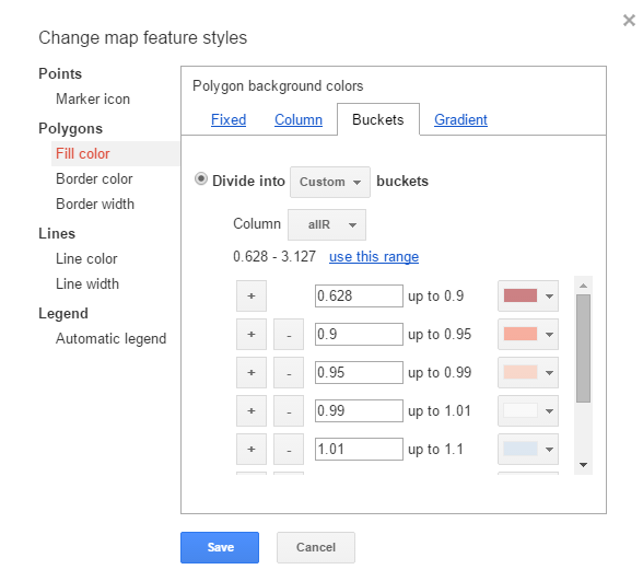
On the left click ‘Change feature styles…’ then Ploygons > Fill color > Buckets. Here you’re on your own to pick the colors to put on the map. Guide to map colors.
And now you’re done! (click Tools > Publish to get code to embed map on your site)
Final map looks like this: